Power BI Blog: ORDERBY Revamped

Welcome
back to this week’s edition of the Power BI blog series.  This week, we consider the changes to ORDERBY and its impact upon associated functions. 
Deep breath – this is a long one!

Back in December last year, the Power
BI updates introduced new functions that make it easier to do comparison
calculations.  Now, these functions are
being made more powerful by adding more control over the ordering of the input
data: the ORDERBY function now accepts any DAX expression as the first
parameter.  Previously, it only accepted
a column (field) name.

As a refresher, that update (first
reported in our February newsletter) saw Microsoft introduce multiple new
functions for DAX, targeted at making it easier to do comparison calculations
in Power BI.  The new functions were as
follows:

• INDEX retrieves a result using absolute positioning
• OFFSET retrieves a result using relative positioning
• WINDOW retrieves a slice of results using absolute or relative positioning.

These functions also come with two
helper functions called ORDERBY (the one that has been updated this
month) and PARTITIONBY. 

These functions will make it easier to
perform calculations such as:

• comparing values against
  a baseline or finding another specific entry (using INDEX)
• comparing values
  against a previous value (using OFFSET)
• adding a running
  total, moving average or similar calculations that rely on selecting a range of
  values (using WINDOW).

If you are familiar with the SQL
language, you will note that these functions are very similar to SQL window
functions.  The functions released in
this update perform a calculation across a set of table rows that are in one
way or another related to the current row.  These functions are different from SQL window
functions, because of the DAX evaluation context concept, which will determine
what is the “current row”.  Moreover, the
functions introduced will not return a value but rather a set of rows which can
be used together with CALCULATE or an aggregation function like SUMX (see elsewhere in this month’s newsletter) to calculate a value.

Further, it should be noted that this
group of functions is not pushed to the data source, but rather they are
executed in the DAX engine.  Additionally,
Microsoft has stated it has seen much better performance using these functions
compared to existing DAX expression to achieve the same result, especially when
the calculation requires sorting by non-continuous columns.

The DAX required to perform these
calculations is simpler than the DAX required without them. However, while
these new functions are very powerful and flexible, they still require a fair
amount of complexity to make them work correctly.  That is because Microsoft opted for high
flexibility for these functions.  However,
the Powers that Be have stated that they recognise there is a need for easier
to use functions that sacrifice some of the flexibility in favour of easier
DAX.  With this in mind, these functions now
released should be seen as “a stepping stone, a building block if you will”
towards Microsoft’s goal to make DAX easier.

To assist what has happened to ORDERBY,
let’s revisit these functions in total.

INDEX

INDEX allows you
to perform comparison calculations by retrieving a row that is in an absolute
position.  This will be most useful for
comparing values against a certain baseline or another specific entry.

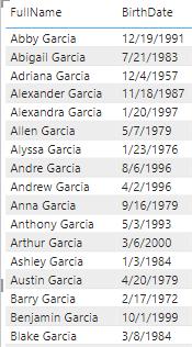
Consider the following example.  Below is a table of customer names and birth
dates whose last name is “Garcia”:

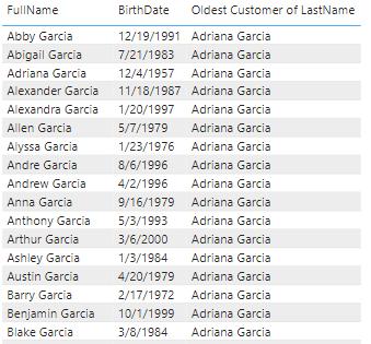
Now, imagine you wanted to find the
oldest customer for each last name.  Therefore,
for the last name “Garcia” that would be Adriana Garcia, born December 4th,
1957.  You can add the following
calculated column on the DimCustomer table to achieve this goal and
return the name:

This would
return the following result: 

In the
example above, we showed only customers whose last name is “Garcia”.  However, the same calculated column works on a
set that has more than one last name:

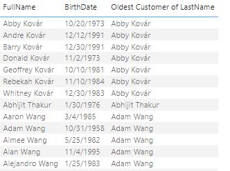
As you can
see in the screenshots above, the full name of the oldest person with that last
name is returned.  That’s because we
instructed INDEX to retrieve the first result when ordering by birth
date, by specifying one [1].  By default,
the ordering for the columns passed into OrderBy is ascending.  If we had specified two [2], we would have
retrieved the name of the second oldest person with the last name instead, and
so on.

Had we
specified -1 or changed the sort order we would have returned the youngest
person instead:

Notice that INDEX relies on two other new helper functions called ORDERBY and PARTITIONBY.

ORDERBY and
PARTITIONBY

These
helper functions may only be used in functions that accept an orderBy or partitionBy parameter, which are the functions introduced above:

• the PARTITIONBY function defines the columns that will be used to partition the rows on which
  these functions operate
• the ORDERBY function defines the columns that determine the sort order within each of a
  window function’s partitions specified by PARTITIONBY.

OFFSET

OFFSET allows you to perform comparison calculations more readily by retrieving
a row that is in a relative position from your current position.  This will be most useful for comparing across
something else than time, for example across regions, cities or products.  For date comparisons, for example, comparing
the sales for this quarter against the same quarter last year there are
dedicated Time Intelligence functions in DAX already.  That doesn’t mean you cannot use OFFSET to do the same, but it is not the immediate scenario.

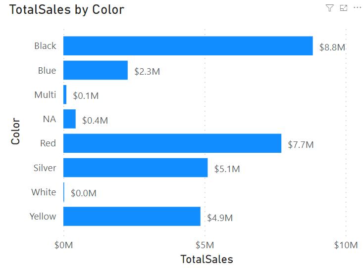
So what is
the scenario for OFFSET?  Consider
the following.  Here’s a Bar chart that
shows total sales by product colour:

Now, let’s
say you wanted to compare how well each colour is doing against the colour
above it in the chart.  You could write a
complicated DAX statement for that, or you can now use OFFSET to
accomplish this goal more simply, viz.

This will
return the following result:

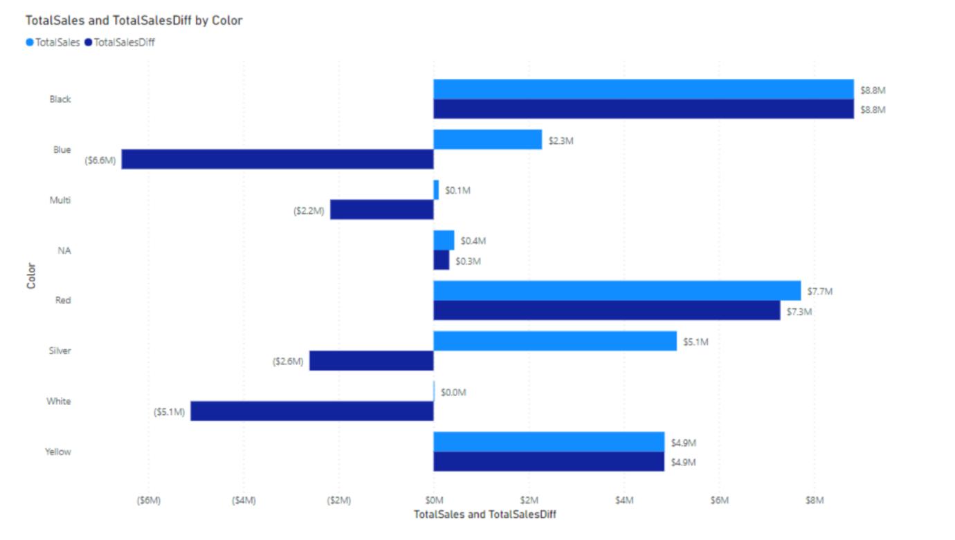
As you can
see the newly added bars calculate the difference for each colour compared to
the one just above it in the chart.  That’s
because the DAX formula specified -1 for the first parameter to OFFSET.  If we had specified -2 we would have made the
comparison against the colour above each colour, but skipping the one right
above it, so effectively the sales for the grey colour would have been compared
against the sales for products that were black, etc.

WINDOW

WINDOW allows you to perform calculations that rely on ranges of results
(“windows”), such as a moving average or a running sum.  For example, the below Column chart shows
total sales by year and month:

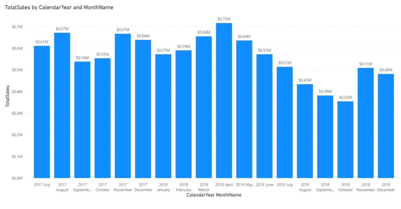
Now, let’s
say you wanted to add a moving average for the last three months of sales
including the current.  For example, for
September 2017, you would expect the result to be the average sales of July,
August and September in 2017 and for February 2018, we would expect the result
to be the average sales for December 2017, January 2018 and February 2018.

To meet
this requirement, you could write a complicated DAX statement or you can now
use WINDOW to accomplish this goal using a simpler DAX statement:

This will
return the following result:

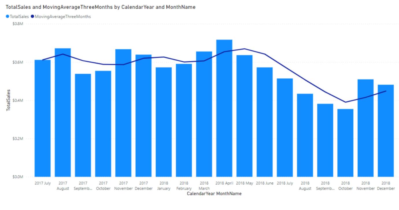
The newly
added line correctly calculates the average sales over three months (including
the current month).  This release on a
so-called ‘relative window’: the first parameter to WINDOW is set to -2,
which means that the start of the range is set two months before to the current
month (if that exists).  The end of the
range is inclusive and set to zero [0], which means the current month.  Absolute windows are available as well, as
both the start and end of the range can be defined in relative or absolute
terms.  Notice that WINDOW relies
on two other new functions called ORDERBY and PARTITIONBY too.

So let’s return to this month’s update.Continuing from the examples above, let’s
figure out which customer has bought the most and return their full name using
the following expression:

Notice how the first parameter of the ORDERBY function is an expression returning the sum of SalesAmount.  This is not something that was possible
before.  We could have performed the same
using a measure defined as:

The BiggestSpender definition then
changes slightly:

In the
meantime, please remember we offer training in Power BI which you can find out
more about here.  If you wish to catch up on past articles, you
can find all of our past Power BI blogs here.