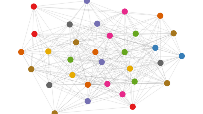
To refine our solutions obtained using heuristics and try to prove the optimality of solutions, let us formulate the Graph Coloring Problem as an ILP model. Remember it might be unable to handle large instances though. The model presented in this section and other exact algorithms are presented in Chapter 3 of Lewis (2021).
Let us define the Sets considered in this approach:
- C: Colors
- N: Nodes (or vertices)
- E: Edges
A first question already comes up “How many colors should we consider?”. In the worst-case scenario, all nodes are connected, so one should consider C of the same size as N. However, this approach could make our solutions even harder by unnecessarily increasing the number of decision variables and worsening the linear relaxation of the model. A good alternative is to use a heuristic method (such as DSatur) to obtain an upper bound for the number of colors.
In this problem, we have two groups of decision variables:
- x_{i, c}: Are binary variables indicating that node i is colored in c
- y_{c}: Are binary variables indicating that color c is used
We must also create constraints to ensure that:
- Every node must be colored
- If any node from one edge has a color, ensure that the color is being used
- At most 1 node of each edge can be colored with a given color
- Break symmetry (this is not required, but might help)
Finally, our objective should minimize the total number of colors used, which is the sum of y. Summarizing we have the following equations.
Without further ado, let us import pyomo for the Integer Programming model.
import pyomo.environ as pyo
There are two approaches for modeling a problem in pyomo: Abstract and Concrete models. In the first approach, the algebraic expressions of the problem are defined before some data values are supplied, whereas, in the second, the model instance is created immediately as its elements are defined. You can find more about these approaches in the library documentation or in the book by Bynum et al. (2021). Throughout this article, we will adopt the Concrete model formulation.
model = pyo.ConcreteModel()
Then, let us instantiate our Sets. Parsing the iterables directly from dsatur attributes N and C is valid, so one could use them in the initialize keyword arguments. Alternatively, I will pass the original nodes and edges from our input data and create a range from the DSatur as our initialization for colors.
model.C = pyo.Set(initialize=range(len(dsatur.C)))  # Colors
model.N = pyo.Set(initialize=nodes)  # Nodes
model.E = pyo.Set(initialize=edges])  # Edges
Next, we instantiate our decision variables.
model.x = pyo.Var(model.N, model.C, within=pyo.Binary)
model.y = pyo.Var(model.C, within=pyo.Binary)
And then our constraints.
# Fill every node with some color
def fill_cstr(model, i):
return sum(model.x[i, :]) == 1# Do not repeat colors on edges and indicator that color is used
def edge_cstr(model, i, j, c):
return model.x[i, c] + model.x[j, c] <= model.y[c]
# Break symmetry by setting a preference order (not required)
def break_symmetry(model, c):
if model.C.first() == c:
return 0 <= model.y[c]
else:
c_prev = model.C.prev(c)
return model.y[c] <= model.y[c_prev]
model.fill_cstr = pyo.Constraint(model.N, rule=fill_cstr)
model.edge_cstr = pyo.Constraint(model.E, model.C, rule=edge_cstr)
model.break_symmetry = pyo.Constraint(model.C, rule=break_symmetry)
You can try and include other symmetry-breaking constraints and see what works better with your available solver. In some experiments I performed, including a preference order using total nodes assigned to a given color has been worse than ignoring it. Possibly due to the solver’s native symmetry-breaking strategies.
# Break symmetry by setting a preference order with total assignments
def break_symmetry_agg(model, c):
if model.C.first() == c:
return 0 <= sum(model.x[:, c])
else:
c_prev = model.C.prev(c)
return sum(model.x[:, c]) <= sum(model.x[:, c_prev])
At last, the objective…
# Total number of colors used
def obj(model):
return sum(model.y[:])model.obj = pyo.Objective(rule=obj)
And our model is ready to be solved! To do that I’m using the HiGHS persistent solver, which is available in pyomo in case highspy is also installed in your Python environment.
solver = pyo.SolverFactory("appsi_highs")
solver.highs_options["time_limit"] = 120
res = solver.solve(model)
print(res)
For large instances, our solver might have a hard time trying to improve heuristic solutions. However, for a 32-node instance available in the code repository, the solver was able to reduce the number of used colors from 9 to 8. Worth mentioning that it took 24 seconds to complete execution whereas the DSatur algorithm for the same instance took only 6 milliseconds (using pure Python, which is an interpreted language).

Be the first to comment