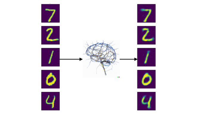
Autoencoders are a fundamental concept in machine learning, particularly in the field of neural networks. Think of them as clever tools that help us compress and then expand data, like squeezing and stretching a rubber ball. Here’s a simple way to grasp what autoencoders do:
Imagine you have a collection of images, but you want to reduce their size while keeping the important details intact. Autoencoders can help with this. They consist of two parts: an encoder and a decoder. The encoder shrinks the image, like squishing it into a tiny version, which represents the compressed information. Then, the decoder takes this compact representation and tries to expand it back into the original image. The magic happens in the training process, where the autoencoder learns to do this compression and decompression efficiently, finding a balance between keeping the essential features and reducing the size. This makes them handy for tasks like image compression, denoising, and feature extraction.
Autoencoders aren’t just limited to images; they can work with various types of data, like text or numerical values. Think of them as a versatile tool to uncover patterns and reduce data complexity. By teaching an autoencoder to compress and then expand your data effectively, you enable it to learn valuable representations, making it a useful addition to your machine learning toolbox. Whether you’re interested in reducing data dimensions or extracting meaningful features, autoencoders are a powerful technique to explore and understand.
So, now that we know what an autoencoder is, how do we build it? We can think of an autoencoder as a neural network itself with an input layer, encoding layer, decoding layer, and then an output layer.
In our basic example, we are going to build one with just a single encoder and decoder layer and then we will feed some standard images into it.
In the end, we will have something which closely resembles the diagram below:
First, let’s import our necessary libraries:
We will be using:
- Keras as our machine learning library and for things like layers, neural network inputs, datasets, etc.
- Numpy for array / matrix operations
- Matplotlib to display results
- Typing for type hints
All dependencies can be found in the requirements.txt.
Next, let’s create a function to build our autoencoder:
This function is relatively simple, actually! Let’s see what we are doing. First, we create an input image using the keras.Input object. This will be the original image that we want our autoencoder to break down and reconstruct.
Next, we create an encoding layer using keras.layers.Dense. The encoded layer will output image representations that are dimensions in size (for example, 32 units). It will also use relu as its activation layer. Finally, we just pass it the input object as input, essentially connecting an input layer to a encoding layer.
Now, we need to make the decoding layer. We want the output dimensions of the decoding layer to be the same dimensions of the original image, so we will use whatever our original image size was. We will also use sigmoid as the activation function here, and then pass it the encoded layer as input. Again, connecting the two layers. Finally, we can put everything together in a keras.Model object with the original input as the model’s input and the output of the decoding layer as the model’s output. Finally, we can just compile the model and return our new autoencoder.
Now that we have some function to create an autoencoder, we need to grab some input data, generate and train our autoencoder, and then do some visual testing to see what it actually does! Let’s first load our mnist data and normalize it for our model (if you’re curious about why to normalize data, here’s a great medium post):
So, we see that we use the keras.datasets.mnist dataset as our dataset. We can load it right into our x_train and x_test variables just by using load_data(). Then, we normalize the values between 0 and 1 and reshape them into vectors of the size of the image (784 for mnist because images are 28×28 and 28 * 28 = 784).
Next, we can go right into our encoder generation and training:
We used our generate_auto_encoder function from before to generate us an autoencoder! Then, we trained the model using the keras API on the training mnist data for a set number of epochs using a set batch size. At this point, we can now go and manually validate how our autoencoder does at deconstruction and reconstruction of images:
First, we call autoencoder.predict() on our testing data to deconstruct and reconstruct each image in our testing dataset. Then, we use matplotlib to plot the original images on the left side of the plot and the reconstructed images on the right side of the plot.
Finally, let’s give this thing a run to see:
- An example output in the terminal
- What the reconstructed images look like
And an example output can be seen below!
The output images should look similar to the inputs, but you’ll notice that they are a bit blurrier. The features that remain are the features that your autoencoder deemed the most important, so there is some loss there (i.e. lossy compression). However, this reduced dimensionality can have some benefits to other neural networks that come next in your image processing/classification pipeline!
All code can be found here on github!

Be the first to comment