Do All the Roads Lead to Rome?. Quantifying the Ancient Question with… | by Milan Janosov | Oct, 2023

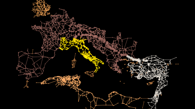
After enjoying the visuals, let’s get back to the graph itself and quantify it. Here, I will compute the total degree of each node, measuring the number of connections it has, and the unnormalized betweenness centrality of each node, counting the total number of shortest paths crossing each node.

node_degrees = dict(G_clean2.degree)
node_betweenness = dict(nx.betweenness_centrality(G_clean2, normalized = False))

Now, I have the importance scores of each crossing. Additionally, in the nodes table, we also have their location — now it’s time to go for the main question. For this, I quantify the importance of each node falling into the admin boundaries of Rome. For this, I will need the admin boundaries of Rome, which is relatively easy to get from OSMnx (note: Rome today is probably different from Rome back in the day, but approximatively, it should be fine).

admin = ox.geocode_to_gdf('Rome, Italy')
admin.plot()

The output of this cell:

Also, on the visuals, it’s pretty clear that Rome is not there as a single node in the road network; instead, many are nearby. So we ned some sort of binning, spatial indexing, which helps us group all road network nodes and intersections belonging to Rome. Additionally, this aggregation would be desired to be comparable across the Empire. This is why, instead of just mapping nodes into the admin area of Rome, I will go for Uber’s H3 hexagon binning and create hexagon grids. Then, map each node into the enclosing hexagon and compute the aggregated importance of that hexagon based on the centrality scores of the enclosed network nodes. Finally, I will discuss how the most central hexagons overlay with Rome.

First, let’s get the admin area of the Roman Empire in an approximative way:

import alphashape # version:  1.1.0
from descartes import PolygonPatch
# take a random sample of the node points
sample = nodes.sample(1000)
sample.plot()
# create its concave hull
points = [(point.x, point.y) for point in sample.geometry]
alpha = 0.95 * alphashape.optimizealpha(points)
hull = alphashape.alphashape(points, alpha)
hull_pts = hull.exterior.coords.xy
fig, ax = plt.subplots()
ax.scatter(hull_pts[0], hull_pts[1], color='red')
ax.add_patch(PolygonPatch(hull, fill=False, color='green'))

The output of this cell:

Let’s split the Empire’s polygon into a hexagon grid:

import h3 # version: 3.7.3
from shapely.geometry import Polygon # version: 1.7.1
import numpy as np # version: 1.22.4
def split_admin_boundary_to_hexagons(polygon, resolution):
coords = list(polygon.exterior.coords)
admin_geojson = {"type": "Polygon",  "coordinates": [coords]}
hexagons = h3.polyfill(admin_geojson, resolution, geo_json_conformant=True)
hexagon_geometries = {hex_id : Polygon(h3.h3_to_geo_boundary(hex_id, geo_json=True)) for hex_id in hexagons}
return gpd.GeoDataFrame(hexagon_geometries.items(), columns = ['hex_id', 'geometry'])
roman_empire = split_admin_boundary_to_hexagons(hull, 3)
roman_empire.plot()

Result:

Now, map the road network nodes into hexagons and attach the centrality scores to each hexagon. Then. I aggregate the importance of each node within each hexagon by summing up their number of connections and the number of shortest paths crossing them:

gdf_merged = gpd.sjoin(roman_empire, nodes[['geometry']])
gdf_merged['degree'] = gdf_merged.index_right.map(node_degrees)
gdf_merged['betweenness'] = gdf_merged.index_right.map(node_betweenness)
gdf_merged = gdf_merged.groupby(by = 'hex_id')[['degree', 'betweenness']].sum()
gdf_merged.head(3)

Finally, combine the aggregated centrality scores with the hexagon map of the Empire:

roman_empire = roman_empire.merge(gdf_merged, left_on = 'hex_id', right_index = True, how = 'outer')
roman_empire = roman_empire.fillna(0)

And visualize it. In this visual, I also add the empty grid as a base map and then color each grid cell based on the total importance of the road network nodes within. This way, the coloring will highlight the most critical cells in green. Additionally, I added the polygon of Rome in white. First, colored by degree:

f, ax = plt.subplots(1,1,figsize=(15,15))
gpd.GeoDataFrame([hull], columns = ['geometry']).plot(ax=ax, color = 'grey', edgecolor = 'k', linewidth = 3, alpha = 0.1)
roman_empire.plot(column = 'degree', cmap = 'RdYlGn', ax = ax)
gdf.plot(ax=ax, color = 'k', linewidth = 0.5, alpha = 0.5)
admin.plot(ax=ax, color = 'w', linewidth = 3, edgecolor = 'w')
ax.axis('off')
plt.savefig('degree.png', dpi = 200)

Result: