Gaussian Processes (GPs) are an incredible class of models. There are very few Machine Learning algorithms that give you an accurate measure of uncertainty for free while still being super flexible. The problem is, GPs are conceptually really difficult to understand. Most explanations use some complex algebra and probability, which is often not useful to get an intuition for how these models work.
There also are many great guides that skip the maths and give you the intuition for how these models work, but when it comes to using GPs yourself, in the right context, my personal belief is that surface knowledge won’t cut it. This is why I wanted to walk through a bare-bones implementation, from scratch, so that you get a clearer picture of what’s going on under the hood of all the libraries that implement these models for you.
I also link my GitHub repo, where you’ll find the implementation of GPs using only NumPy. I’ve tried to abstract from the maths as much as possible, but obviously there is still some that are required…
The first step is always to have a look at the data. We are going to use the monthly CO2 atmospheric concentration over time, measured at the Mauna Loa observatory, a common dataset for GPs [1]. This is intentionally the same dataset that sklearn use in their GP tutorial, which teaches how to use their API and not what is going on under the hood of the model.
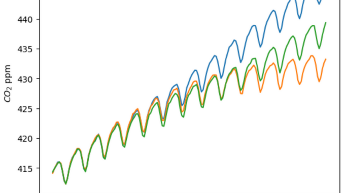
This is a very simple dataset, which will make it easier to explain the maths that will follow. The notable features are the linear upwards trend as well as the seasonal trend, with a period of one year.
What we will do is separate the seasonal component and linear components of the data. To do this, we fit a linear model to the data.

Be the first to comment