Power BI Blog: More on DAX Query View

Welcome back to
this week’s edition of the Power BI blog series.  This week, we look in more detail at the new DAX
query view feature in Power BI Desktop.

The DAX query
view provides a brand new fourth view in public Preview to Power BI Desktop.

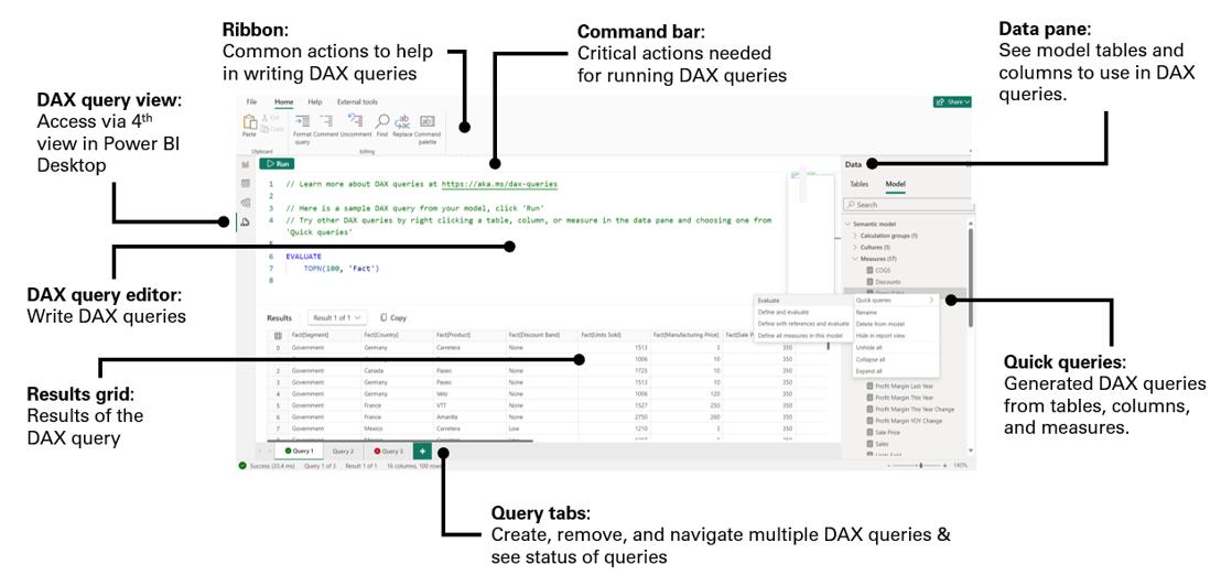
The DAX query view gives you the ability to write, edit and see the results of Data
Analysis eXpressions or DAX queries on your semantic model.  This means you may now take advantage of the
existing DAX queries syntax while working with your semantic model
without leaving Power BI Desktop.

As this feature is
in public Preview, to see the DAX query view in Power BI Desktop, you
need to make sure you are using at least the November 2023 release and have initialised
it via File -> Options and Settings -> Options -> Preview features and then clicked the check box next to ‘DAX query view’.

This new way to
interact with your semantic model in Power BI Desktop comes with several ways
to help you be more productive with DAX queries:

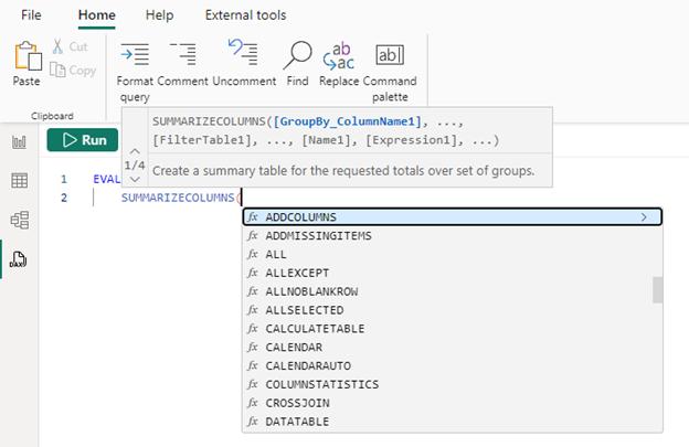
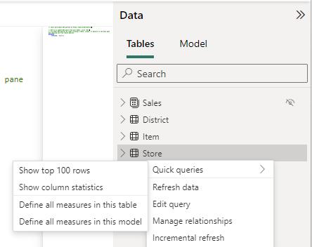
• Quick
  queries from the Data pane makes it easy to create a DAX query.  You may preview
  data or show summary statistics to help you understand the data without needing
  to create visuals or writing a DAX query.  You can find quick queries in the context menu
  of tables, columns or measures in the Data pane of the DAX query view
• DirectQuery
  model authors can use DAX query view.  You no longer need to go back to
  Power Query to preview the data
• A new
  measure authoring workflow.  You may now see multiple measures at once in
  the editor, make changes, run the query to test and finally update the model all
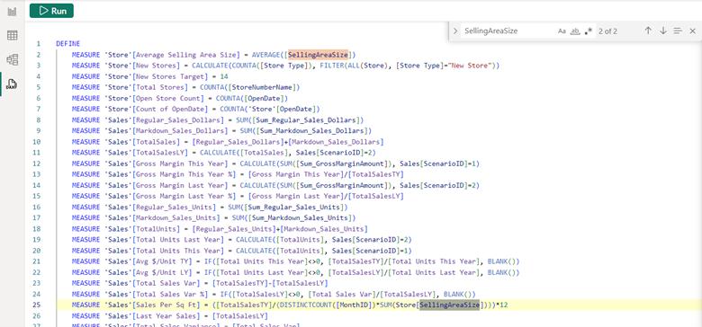
  in one location
• See the DAX
  query of the visuals.  If a particular Power BI visual is not showing
  the data you expect, you may now investigate further by looking at the DAX query
  used by the visual to get data.  This may
  be accessed from the ‘Performance Analyzer’ pane
• Create your
  own DAX query.  You may simply write the DAX query in
  the DAX query view and click run.  You can even define and use measures and
  variables for that DAX query that do not exist in the model.

DAX query view, as the name suggests, allows you to
create DAX queries.  This is
different to the DAX formulae used to create measures and calculated
columns.  A DAX query is like an SQL query in that you can use it to view data in your model.

With this borne in
mind, there are two main parts to a DAX query:

1. EVALUATE: this is required and specifies what data you wish to see
2. DEFINE: this is optional and may specify a measure or named DAX formula
   to use in the DAX query.  This
   measure may already be in the model (it might not be).  If it already exists, you can make changes
   that only apply to this DAX query to try them out.  You can also have the option to update the
   model with these measures (see below).

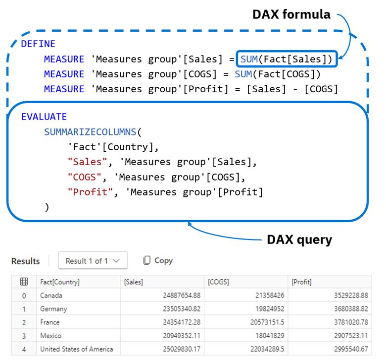
The result of
running a DAX query is a table of data.  

Some of you may
already be familiar with DAX queries from using DAX Studio.  DAX Studio is a community driven and free
external tool that can also run DAX queries.  More than just run DAX queries, it has
plenty of features utilising DAX authoring / performance.  It may be accessed in Power BI Desktop from
the External tools Ribbon once installed.

DAX query view can generate examples for you so that
you may see a DAX query, run it,and modify it as needed.  Here’s an example using Quick queries.

Microsoft provide
an examples, so that you may follow along. 
You may download the Store Sales PBIX from https://learn.microsoft.com/power-bi/create-reports/sample-datasets#updated-samples.

When you first
click on DAX query view, a sample query is shown to get the top 100 rows
of one of the tables in the model.  In
the case of Store Sales, this is the Store table.

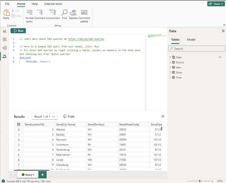
Click Run and the
top 100 rows of the table are shown in the result grid.  In SQL, this is the same as:

This is great to
get a preview of the data for all columns, but it’s difficult to change which
columns you might wish to see.  Therefore,
let’s try ‘Quick queries’ instead.  In
the Data pane, right-click the Store table and from the context menu,
choose Quick queries -> Show top 100 rows.

A new query tab
will be created with a different DAX query showing the same data.  This time, all the columns are explicitly
listed.  There is a TOPN section
which also specifies which column and the order in that column to choose the
top 100 rows, as well as an ORDER BY to specify the result order.

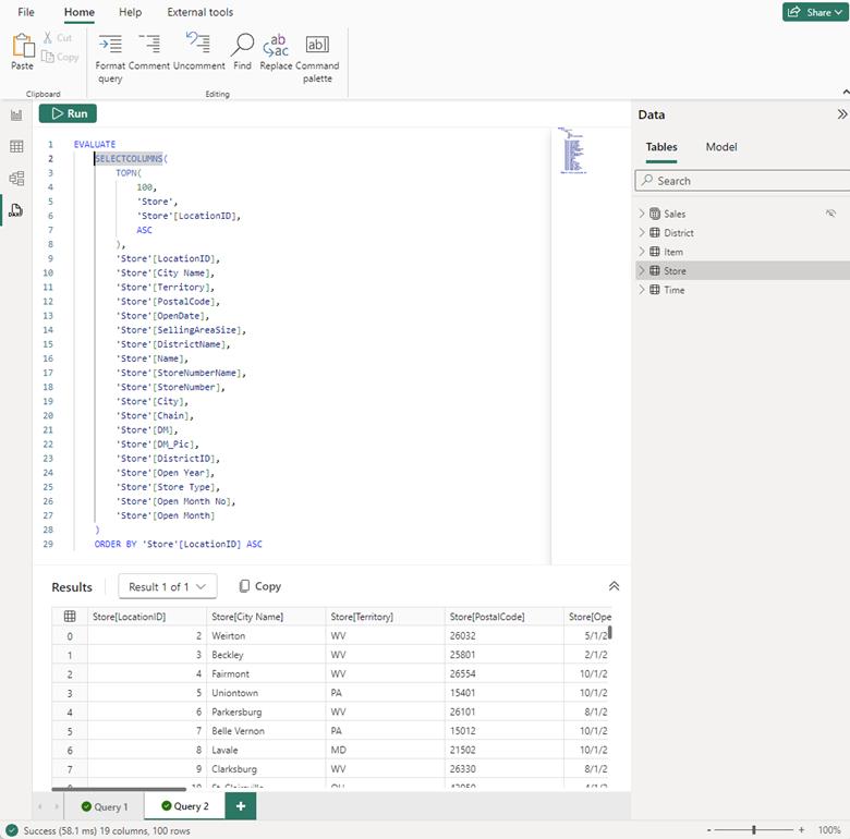
We may now see how SELECTCOLUMNS works to get data from the model.  In
SQL, this would be the same as:

With this quick
query we can remove or comment out columns we don’t want to see in the result
grid, adjust the number of rows, change the order by column, etc.  SELECTCOLUMNS is used for this query
because if you have multiple rows with the same values, they will all show.  You may change this to SUMMARIZE to
de-duplicate the rows.

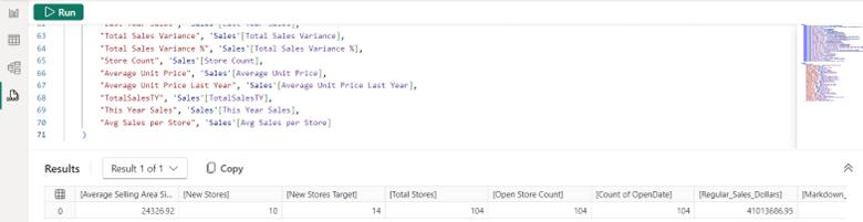
Let’s just look at
the City, Store Name, Store Type and Selling Area Size for each location and order by the Selling Area Size for all rows.  To do this, comment out or remove the unwanted
columns, change TOPN to simply refer to the table and change the column
used in ORDER BY.

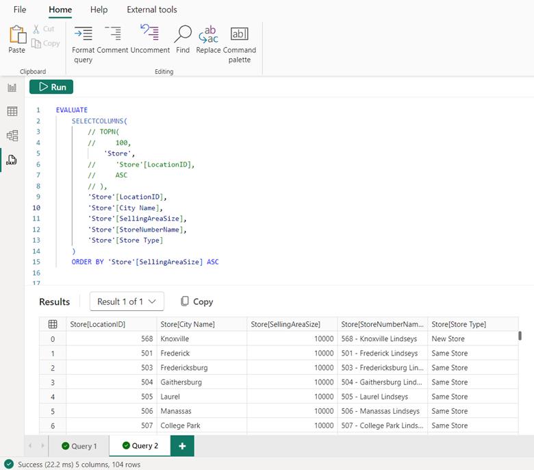
Now, we see
targeted information about all 104 stores.  We may even copy this and paste the results
into Excel.

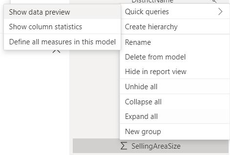
Now, let’s say
we’re curious to see what the possible Selling Area Sizes values are.  This looks like it’s not an exact number, but
instead a way to group stores by size.  In
the Data pane, right-click the SellingAreaSize column and from the
context menu choose Quick queries -> Show data preview.

We can now see
there are nine [9] values for Selling Area Size.  As suspected, this is a way to group stores by
size.

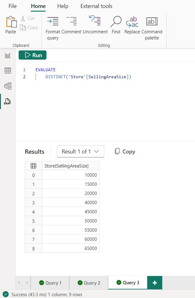
In SQL, this DAX
query is the same as:

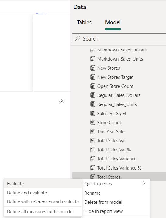
Let’s consider how
many stores we have by each Selling Area Size.  In this data, there is a measure called [Store
Count], so let’s see that number by using a quick query.  It’s easier to find all the measures in the
model by changing to Model in the Data pane, or using the Search bar if you
already know the name.  In the Data pane,
right-click the Store Count measure and from the context menu choose Quick
queries -> Evaluate.

This will create a DAX query again in a new query tab.  Yet
again, we note that there are 104 stores in this data.

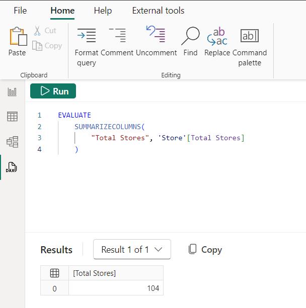
In SQL, there is no
real equivalent to a measure in a semantic model: you have to define the
aggregation in each SQL query, which is instead the same as an implicit measure
in a DAX query.  However, you can
get the same result with this SQL query:

This quick query
uses SUMMARIZECOLUMNS, which means we can add in a group by column, such
as Selling Area Size, to answer the question about how many stores we
have for each store size.

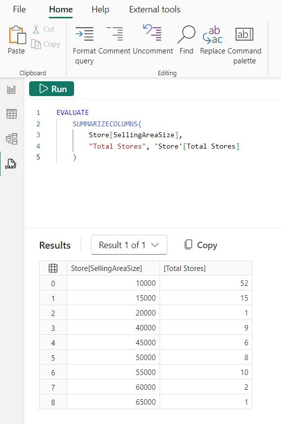
You’ll notice most
of the stores are comparatively small.  We can build on this query even further, not
only by adding in more group by columns, but also by adding in more measures.  Let’s add in Sales.

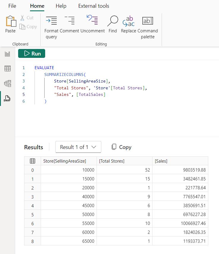
The DAX query view can also show the DAX formula of the [TotalSales] measure.  We may hover over it to see it
in an overlay:

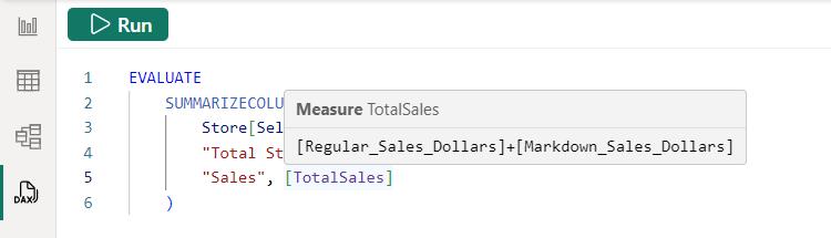
We can see that
it’s referencing other measures in the model.  However, we can’t see their DAX formulae
in the overlay, but DAX query view can take advantage of the DEFINE syntax
in DAX queries.  We may show this
measure’s DAX formula and all referenced measures’ DAX formulae
in just a couple of clicks:

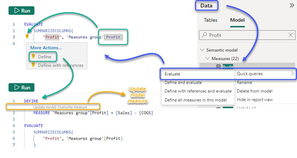
• Click on
  the measure name, placing the cursor in the measure name on line 5.  A lightbulb will appear to the left
• click on
  the lightbulb to see the actions available or use CTRL + . (period)
• click on Define
  with references.

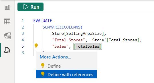
This will create
the DEFINE block for this DAX query just above the EVALUATE.
 These won’t be available if you already
have a DEFINE command in the query tab.

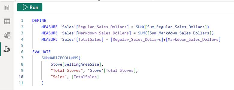
Not only can you
see the DAX formulae, you may even edit one or more of them.  When you run the DAX query, they will
use the modified version in the query tab over the model measure DAX formula.
 This way we can test any changes.  Here, we have doubled one of the measures.  We may even add a measure to use in the DAX query that doesn’t yet exist in the model, such as to see what the average
sales per store is for each store size.

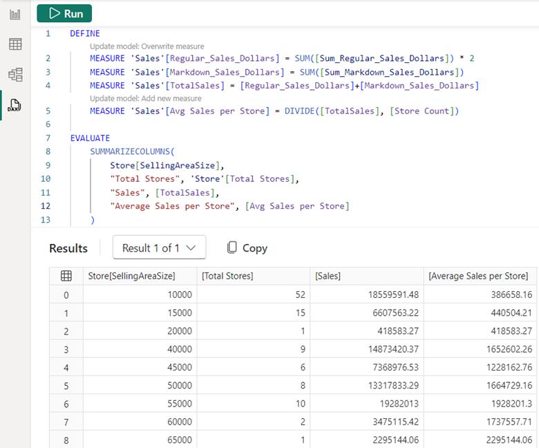
DAX query view can detect when you have changed the DAX formula in a measure that exists in the model, so a clickable superscript
appears, called a CodeLens, which will update the model with the new DAX formula if clicked.  For a measure that
doesn’t already exist in the model, the CodeLens will add this measure
to the model when clicked.  We don’t want
to keep the multiply by two [2] change, but we do want to add in the average
sales per store measure.  The measure is
added to the model and the CodeLens disappears.

We may even remove
the DEFINE block and run the query again.

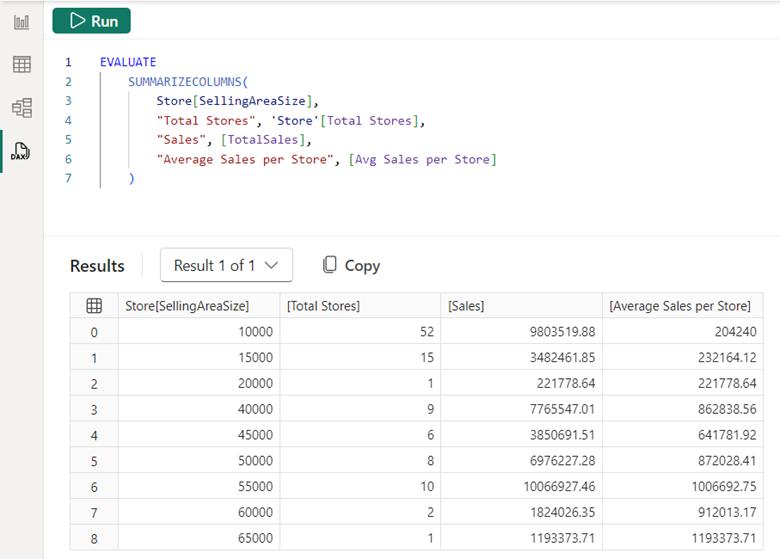
The larger selling
area size of the store does show higher average sales.  The measure quick queries and CodeLenstogether create a new measure authoring workflow in DAX query view.

The quick queries
for measures also has the option to define all the measures in a table or model.  In the Data pane, right-click the any measure
and from the context menu choose Quick queries -> Define all measures in
this model.

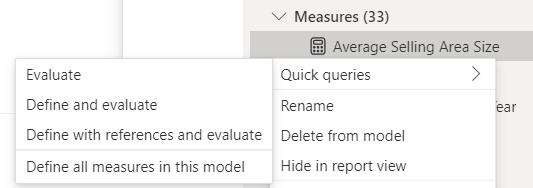
You now have a
large DAX query that defines all the measures and creates an EVALUATE block to see them all at the model level.

SQL again doesn’t
have an equivalent to measures in the semantic model.  These would all need to be aggregations in a
SQL query, but DAX formulae can reference other measures and perform
context changing (looking at last year or by a particular filter) which is more
challenging to reproduce in SQL.

Once we have all our
measures in one single query tab, we can do things such as “find”.  We can see how many measures use the Selling
Area Size column, as an example.  To
do this, we click the ‘Find’ Ribbon button or use CTRL + F.  You will note there are two [2] measures that
are using that column:

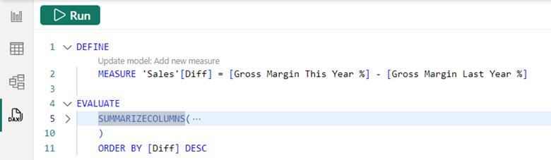
Now we have a feel
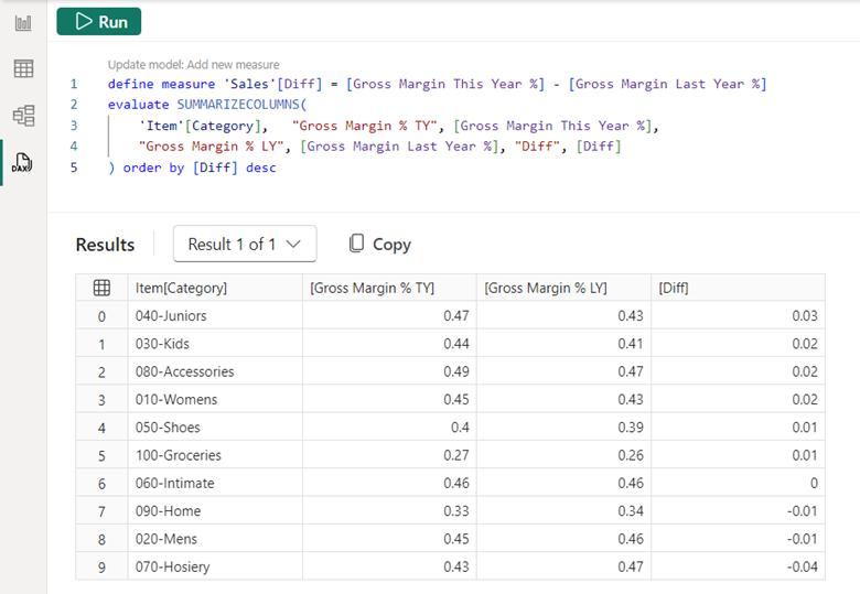
for how DAX queries work, we may create our own.  To start, let’s add a new query tab.  We can use SUMMARIZECOLUMNS to see how
gross margin compares across item categories and then define our own measure to
show the year over year difference and order the results by categories that
improved the most.

We may quickly do
this analysis simply by using DAX queries.  This DAX query doesn’t look as pretty
as the Quick queries, as we typed it by hand not paying attention to the
formatting.  However, we may click the ‘Format
query’ Ribbon button or right-click and choose ‘Format document’ or even use SHIFT
+ ALT + F to format our DAX query.

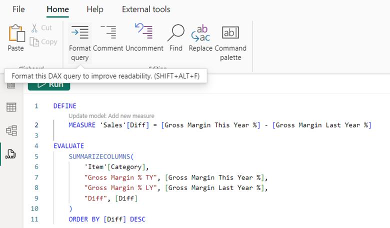
Formatting is more
than just making it pretty looking and easier to read.  We can collapse blocks where they are
indented too.

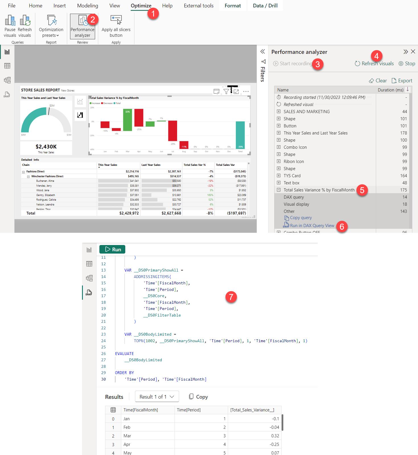
The visuals
themselves are also more than just pretty data visualisations.  The report view visuals get the data from the
model with a DAX query.  It is
possible to see the DAX query in DAX query view as well.  In Report view, go to the ‘Optimize’ Ribbon
and click ‘Performance Analyzer’.  Now,
click ‘Start recording’ followed by ‘Refresh visuals’.  Finally, expand the visual title in the list
and click ‘Run with DAX query view’.  This
will move you to DAX query view where you see the visual DAX query and the results.

In the meantime, please remember we offer training in Power BI which you can find out more about here.  If you wish to catch up on past articles, you can find all of our past Power BI blogs here.